Week 13 - Exploring the data

CHC9012 | National Taiwan Normal University

🎯 Goals

Explore your data:

Non-valid data: How to identify and remove non-valid data?

Analyses: How to analyze and further explore your data?

💻 Dataset and script

Please download the files for the content of Week 13, and place them in your PreprocessingAnalysesR folder.

📥 Download the dataset for the script

📥 Download the R Markdown script

💻 Please start RStudio and select the project called PreprocessingAnalysesR.

💻 Preparations for the analyses

load(file = "CHC9012_PCIbexDataPrepared.RData")

library(ez)
library(dplyr)
library(Rmisc)

👀 Part 1: Have an overview of the results

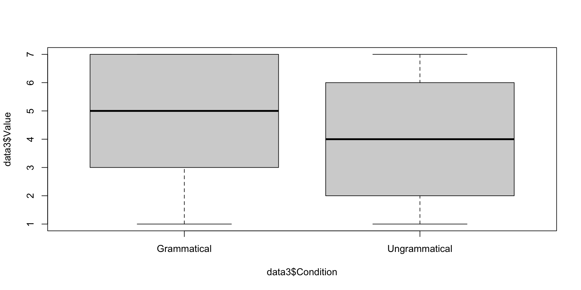
Overall results (1/2)

plot(data3$Value ~ data3$Condition)

Distribution of the ratings across conditions

Please briefly describe the patterns of results.

Overall results (2/2)

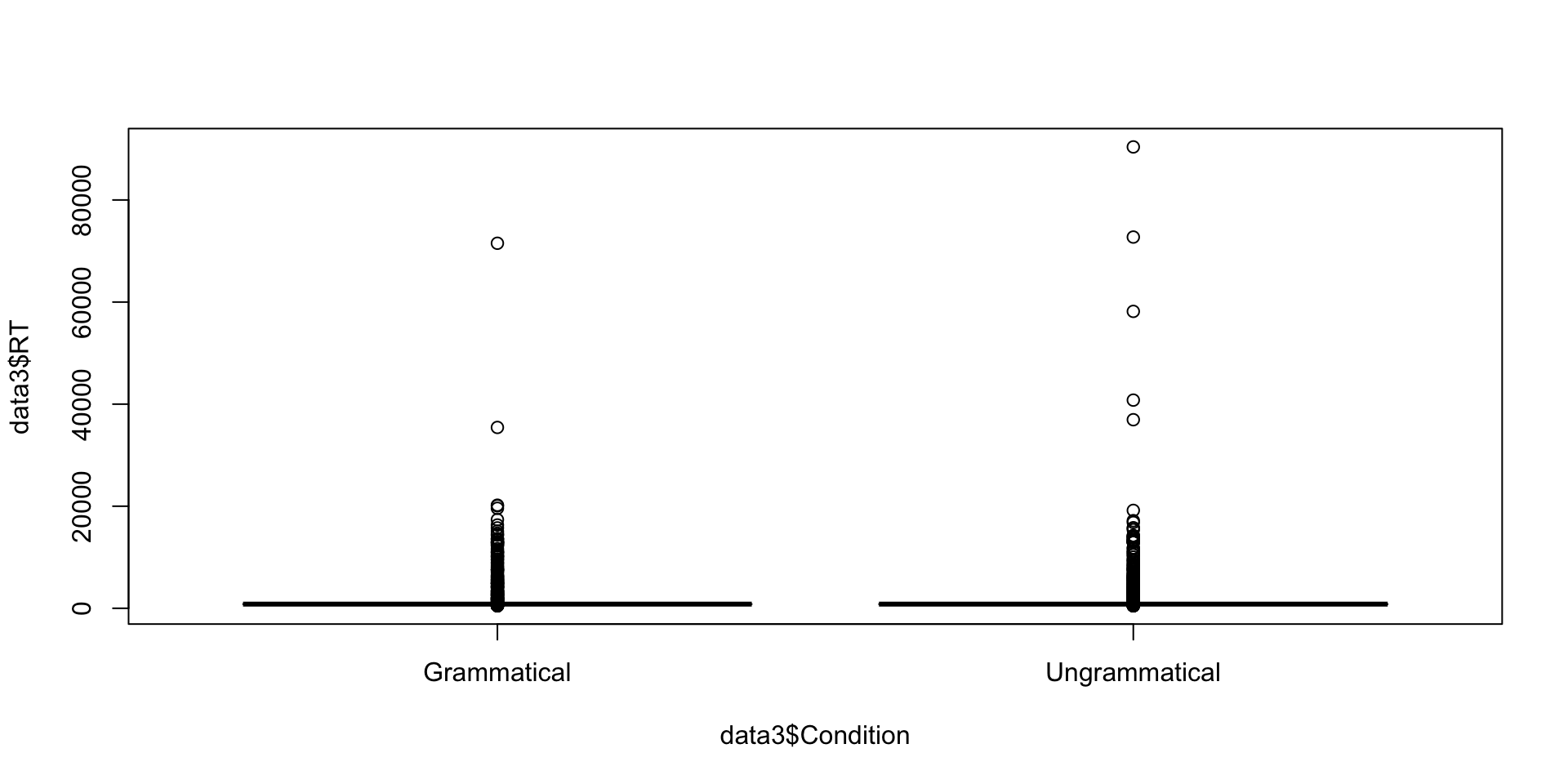
plot(data3$RT ~ data3$Condition)

Distribution of the ratings across conditions

Please briefly describe the patterns of results.

Overall results (2/2)

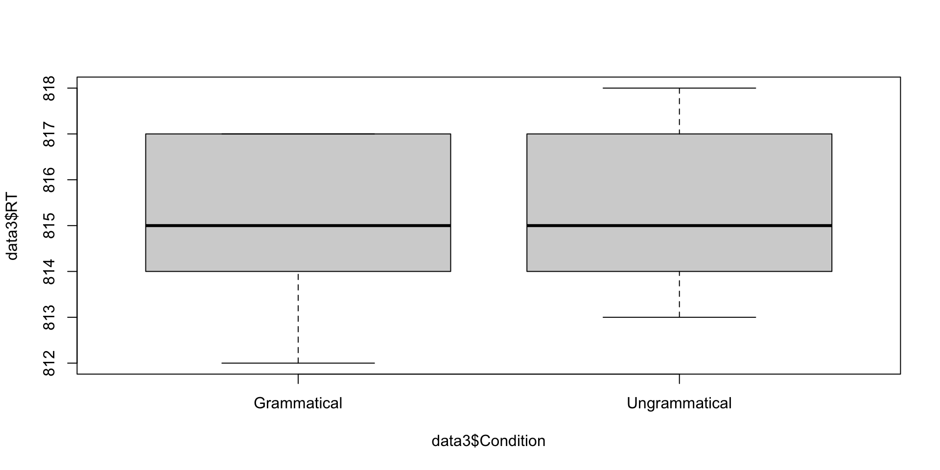
plot(data3$RT ~ data3$Condition, outline = FALSE)

Distribution of the ratings across conditions

Please briefly describe the patterns of results.

Overall results by participant (1/2)

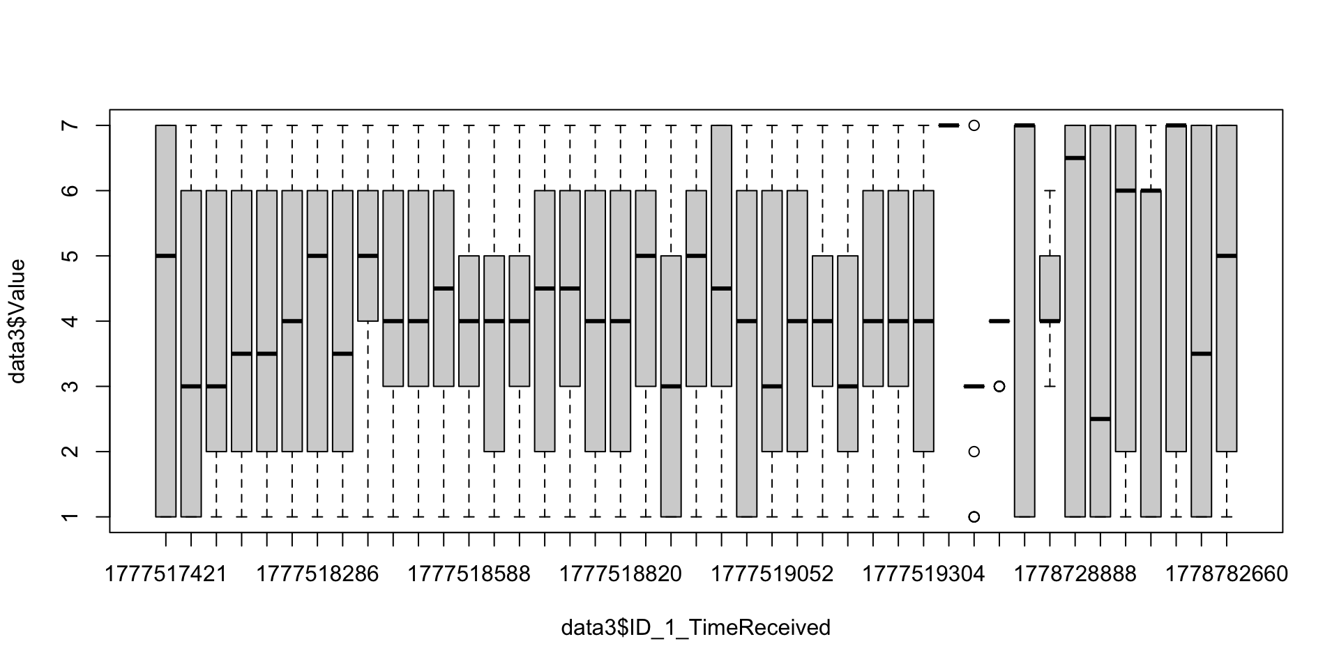
plot(data3$Value ~ data3$ID_1_TimeReceived)

Distribution of the ratings by participants

Are there many very deviant participants?

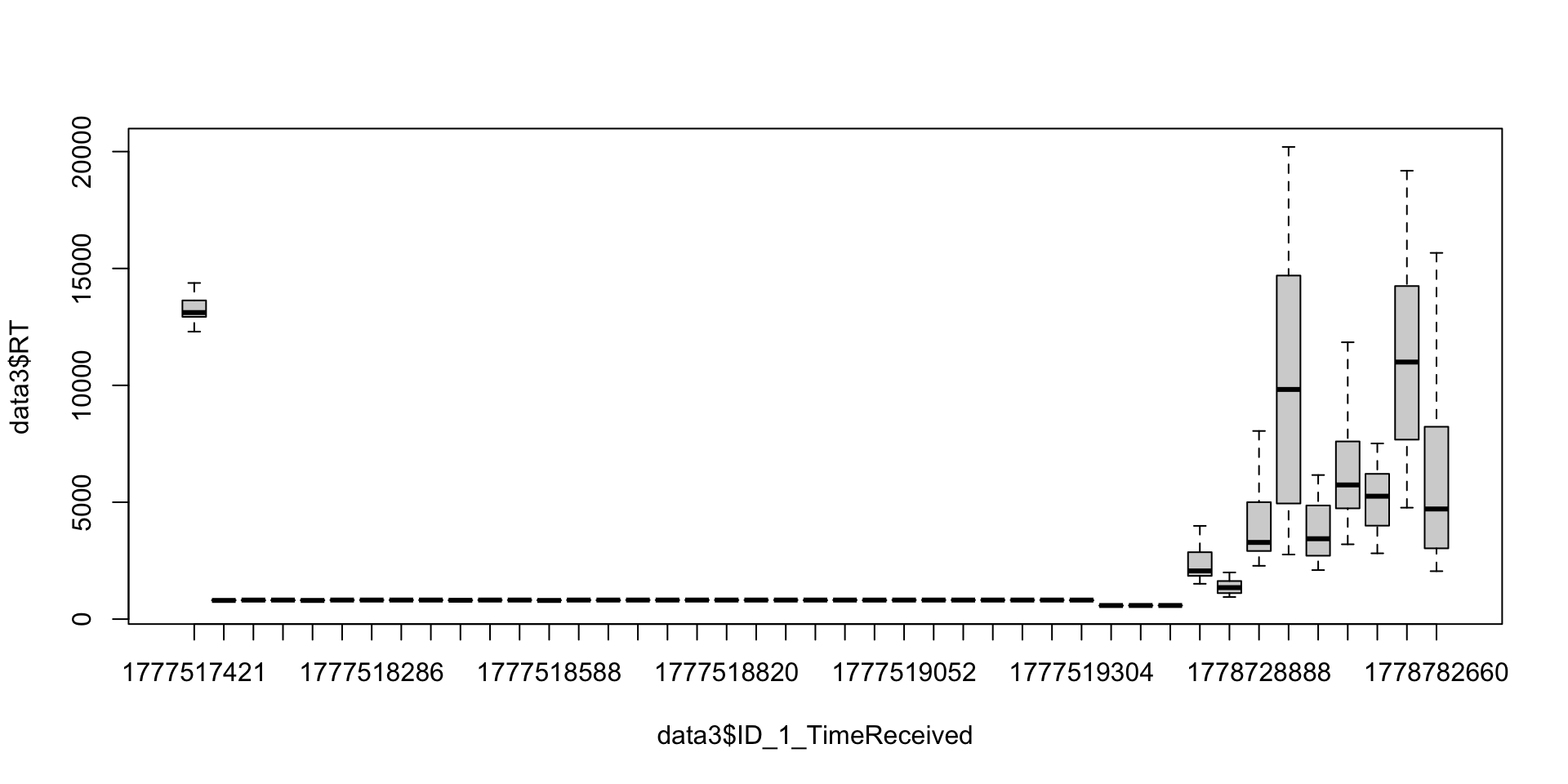
Overall results by participant (2/2)

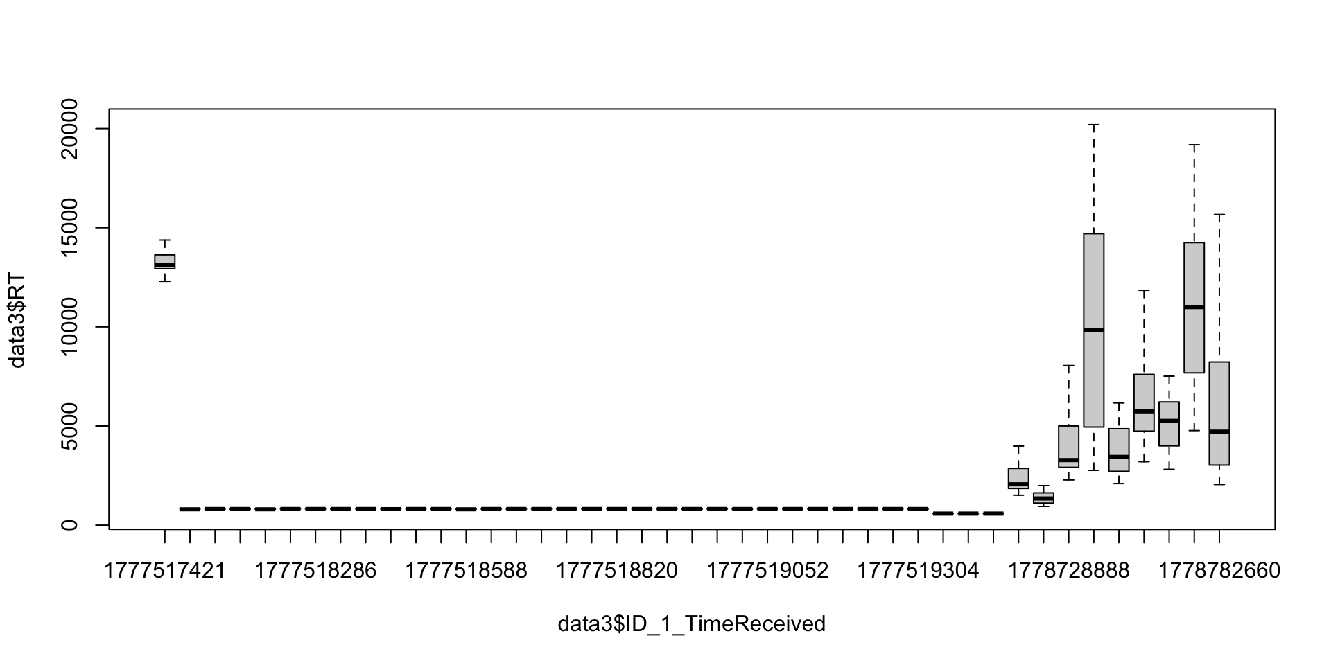
plot(data3$RT ~ data3$ID_1_TimeReceived, outline = FALSE)

Distribution of the ratings by participants

Are there many very deviant participants?

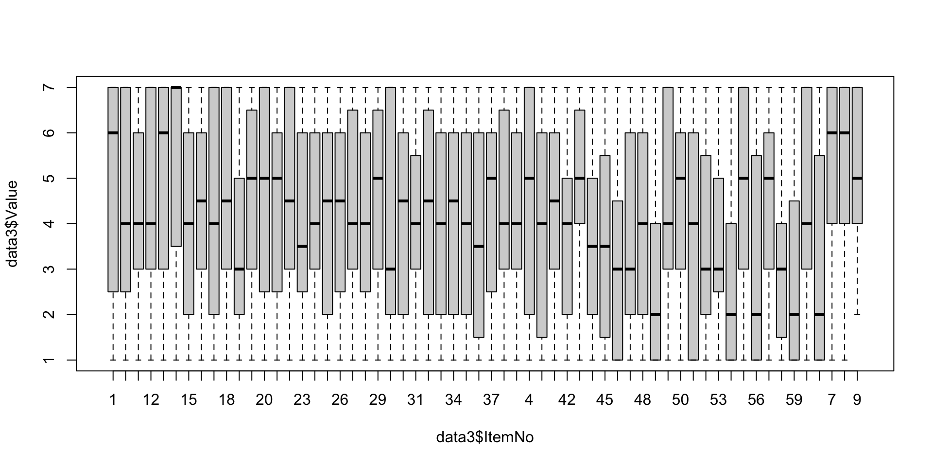
Overall results by item (1/2)

plot(data3$Value ~ data3$ItemNo)

Distribution of the ratings by participants

Are there many very deviant items?

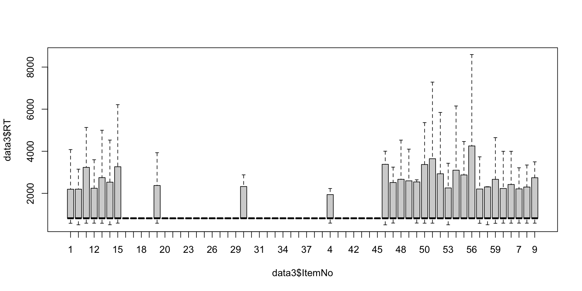
Overall results by item (2/2)

plot(data3$RT ~ data3$ItemNo, outline = FALSE)

Distribution of the ratings by participants

Are there many very deviant items?

How to look at the background of the participants?

Number of participants

length(levels(data3$ID_1_TimeReceived))

[1] 43

Age

summary(data3$UserAge)

   Min. 1st Qu.  Median    Mean 3rd Qu.    Max. 
  19.00   23.00   30.00   35.12   49.00   65.00

Level of education

DegreePart <- subset(data3, select = c(ID_1_TimeReceived, UserDegree))
DegreePart <- unique(DegreePart)
table(DegreePart$UserDegree)


         BA High school          MA       Ph.D. 
         14           7          13           9

Summary

Overall pattern: Grammatical sentences more accepted that ungrammatical ones, but not very obvious

Non-valid data: Many participants with a strange behavior

🤯 Part 2: Identify and remove outliers

2.1. Identify and remove non-valid participants

⚠️ Be careful

We need to be careful when removing data! We need converging evidence and justify our choice.

Different types of evidence to identify non-valid participants:

Based on abnormal mean reaction time

Based on shared IPs (shared device)

Based on the observation of specific participants

Abnormal RT: Overall observations

plot(data3$RT ~ data3$ID_1_TimeReceived, outline = FALSE)

PartMeanRT <- aggregate(RT ~ ID_1_TimeReceived,
                        data = data3,
                        FUN = mean)

print(PartMeanRT)

   ID_1_TimeReceived         RT
1         1777517421 13571.0667
2         1777518106   805.1000
3         1777518142   808.9333
4         1777518178   808.5000
5         1777518214   806.3333
6         1777518250   813.2667
7         1777518286   811.7333
8         1777518322   814.4333
9         1777518359   811.2667
10        1777518398   806.8333
11        1777518439   814.5000
12        1777518549   813.5333
13        1777518588   805.7000
14        1777518627   812.1333
15        1777518665   810.1333
16        1777518704   815.0000
17        1777518742   812.1667
18        1777518781   815.3000
19        1777518820   812.9667
20        1777518859   814.9333
21        1777518898   814.5000
22        1777518937   810.2000
23        1777518975   812.4000
24        1777519013   807.5333
25        1777519052   814.6333
26        1777519104   813.5667
27        1777519142   815.1667
28        1777519180   813.4333
29        1777519233   814.9333
30        1777519270   814.8667
31        1777519304   807.6333
32        1777519458   608.8667
33        1777519500   815.4667
34        1777519539   692.3667
35        1777519798  8069.6667
36        1777952741  1511.9667
37        1778728888  3986.5667
38        1778729203 14339.8000
39        1778730554  4272.8333
40        1778737433  6259.6333
41        1778742733  5526.1333
42        1778763194 11567.2667
43        1778782660  6250.8000

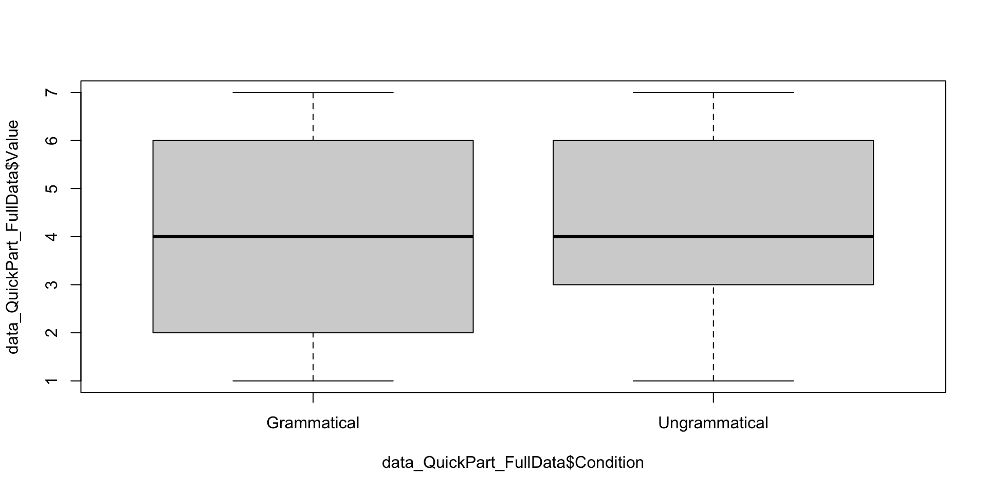
Abnormal RT: Focus on the weird behavior

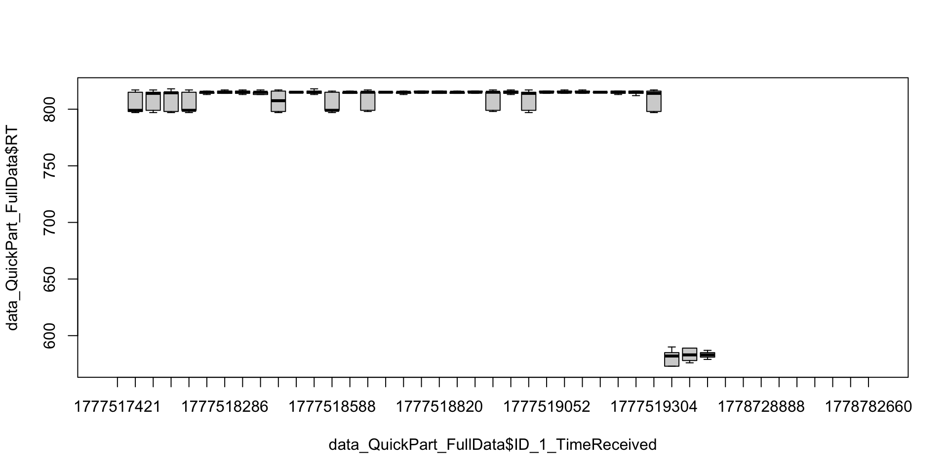
data_QuickPart <- subset(PartMeanRT, RT < 1000)
data_QuickPart_FullData <- subset(data3,
                                  ID_1_TimeReceived %in% data_QuickPart$ID_1_TimeReceived)

plot(data_QuickPart_FullData$RT ~ data_QuickPart_FullData$ID_1_TimeReceived, outline = FALSE)

plot(data_QuickPart_FullData$Value ~ data_QuickPart_FullData$Condition)

Abnormal RT: Focus on the human-like behavior

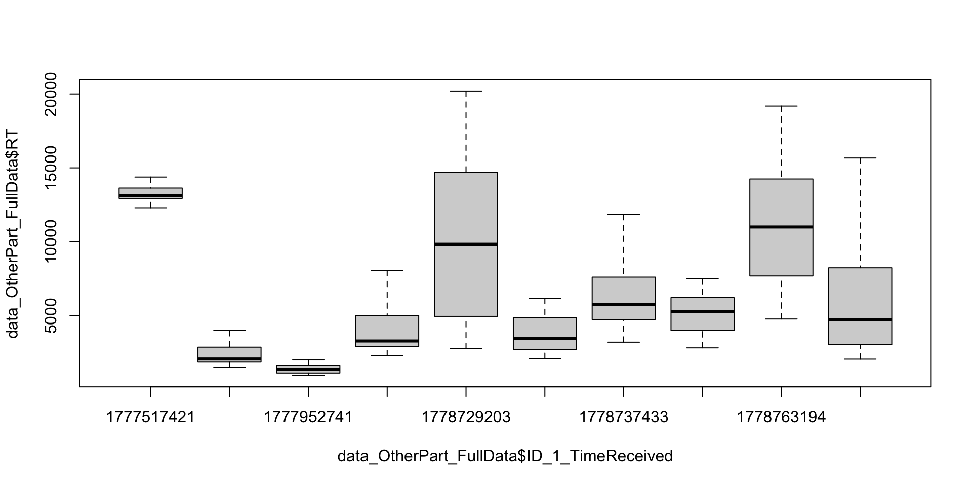
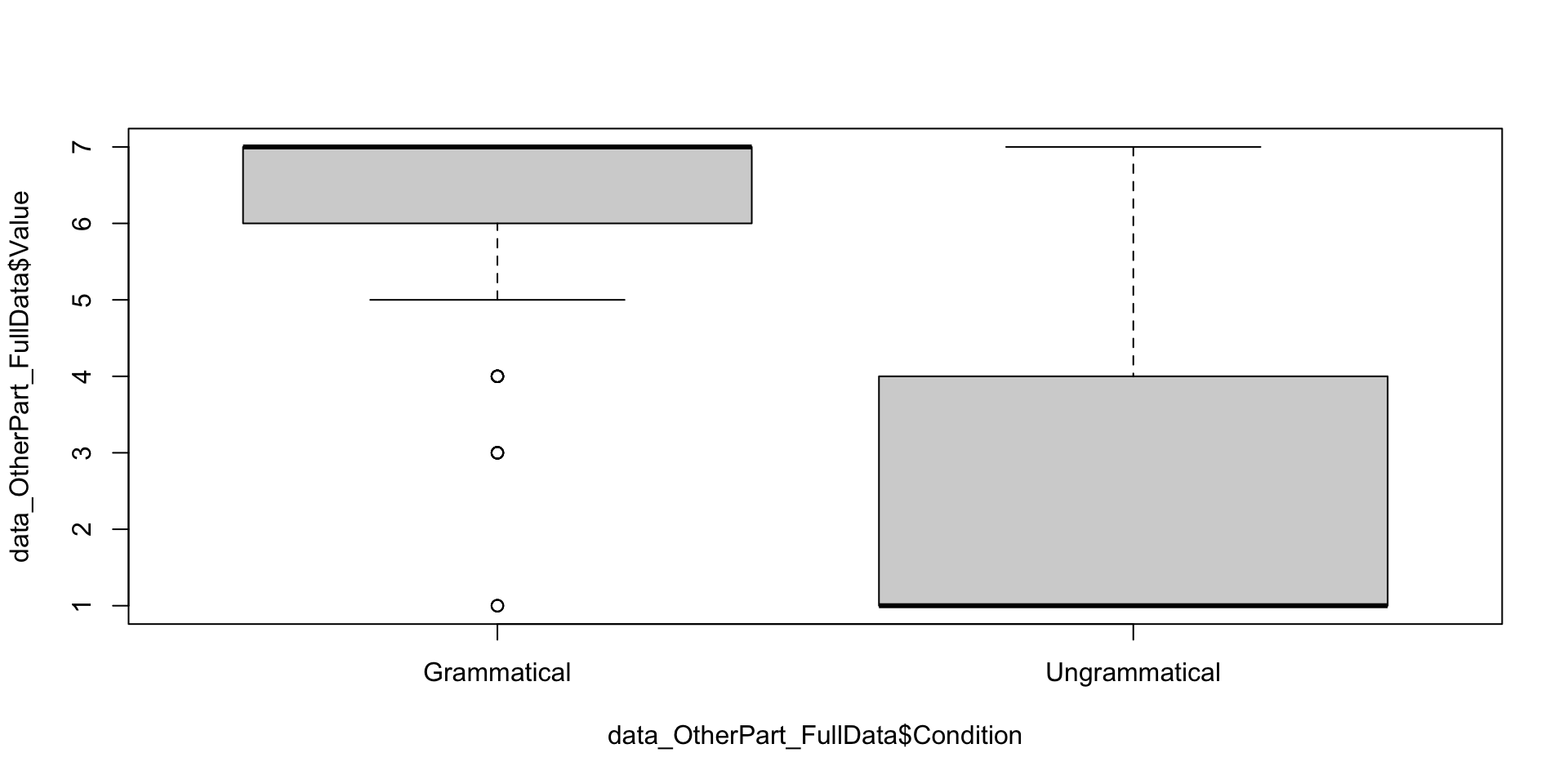
data_OtherPart <- subset(PartMeanRT, RT > 1000)
data_OtherPart_FullData <- droplevels(subset(data3,
                                             ID_1_TimeReceived %in% data_OtherPart$ID_1_TimeReceived))

plot(data_OtherPart_FullData$RT ~ data_OtherPart_FullData$ID_1_TimeReceived, outline = FALSE)

plot(data_OtherPart_FullData$Value ~ data_OtherPart_FullData$Condition)

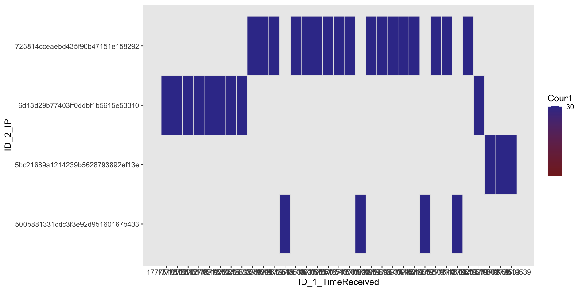
Shared IPs (shared device)

Weird RTs

ezDesign(data_QuickPart_FullData,
ID_1_TimeReceived,
ID_2_IP)

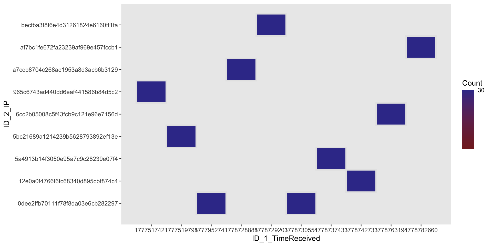
Human-like behavior

ezDesign(data_OtherPart_FullData,
ID_1_TimeReceived,
ID_2_IP)

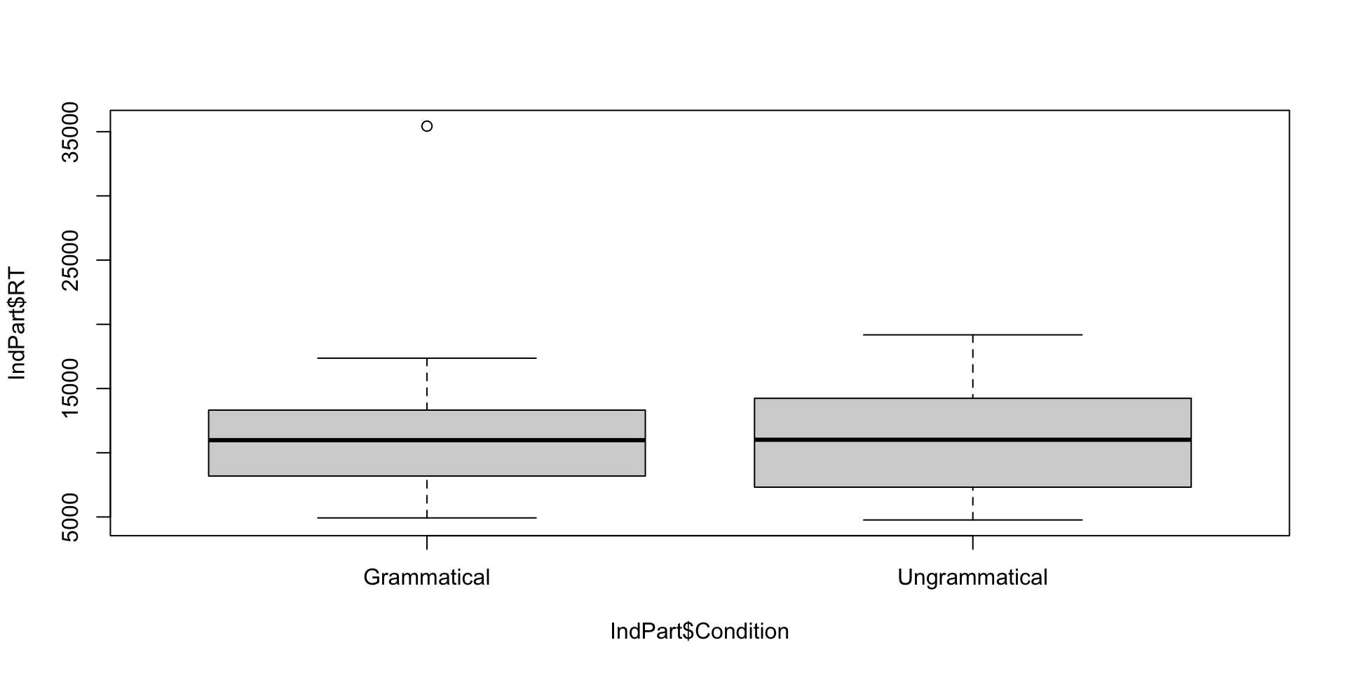
Look at specific participants

Code to extract the data of one participant (here, Participant #9)

IndPart <- subset(data_OtherPart_FullData,
                  ID_1_TimeReceived == levels(data_OtherPart_FullData$ID_1_TimeReceived)[9])

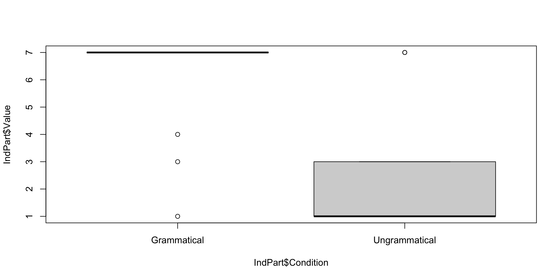
plot(IndPart$Value ~ IndPart$Condition)

plot(IndPart$RT ~ IndPart$Condition)

Summary

Converging evidence to say that one group’s behavior is very different, indicating that they did not pay attention to the task

Further analyses: Inclusion of participants with the human-like behavior

2.2. Identify and remove non-valid trials

Remove based on absolute values

data_OtherPart_CleanAbsolute <- subset(data_OtherPart_FullData, RT > 200 & RT < 20000)

Remove based on relative values (1/2)

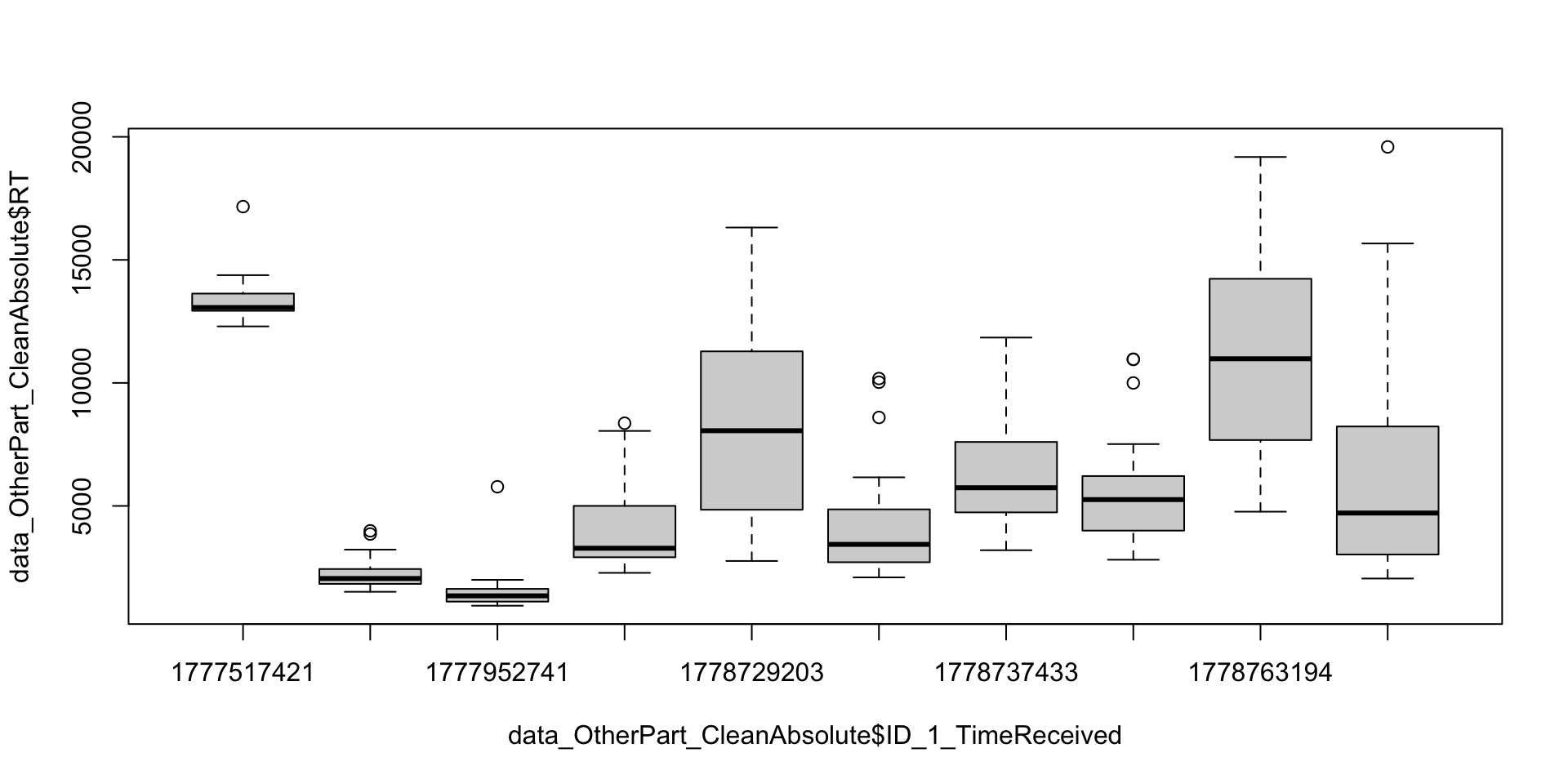
plot(data_OtherPart_CleanAbsolute$RT ~ data_OtherPart_CleanAbsolute$ID_1_TimeReceived)

Remove based on relative values (2/2)

# Calculate the mean per Participant and Condition
data_OtherPart_CleanAbsolute$m_rt <- ave(data_OtherPart_CleanAbsolute$RT, 
                                         data_OtherPart_CleanAbsolute$ID_1_TimeReceived, 
                                         data_OtherPart_CleanAbsolute$Condition, 
                                         FUN = mean)

# 2. Calculate the SD per Participant and Condition
data_OtherPart_CleanAbsolute$sd_rt <- ave(data_OtherPart_CleanAbsolute$RT, 
                                          data_OtherPart_CleanAbsolute$ID_1_TimeReceived, 
                                          data_OtherPart_CleanAbsolute$Condition, 
                                          FUN = sd)

# 3. Subset the data to remove outliers
data_OtherPart_CleanAbsoluteRelative <- subset(data_OtherPart_CleanAbsolute, 
                                               RT >= (m_rt - 2.5 * sd_rt) & 
                                                 RT <= (m_rt + 2.5 * sd_rt))

Calculate the proportion of removed trials

FullData_NbTrials <- nrow(data_OtherPart_FullData)
TrimmedData_NbTrials <- nrow(data_OtherPart_CleanAbsoluteRelative)

# Number of trimmed trials
NbTrimmedTrials <- FullData_NbTrials - TrimmedData_NbTrials
NbTrimmedTrials

# Proportion (%)
NbTrimmedTrials*100/FullData_NbTrials

[1] 14

[1] 4.666667

The proportion is below 5%, which is acceptable in experimental linguistics.

📊 Part 3: Analyses and explorations of the clean results

3.1: Design-based analyses: Ratings

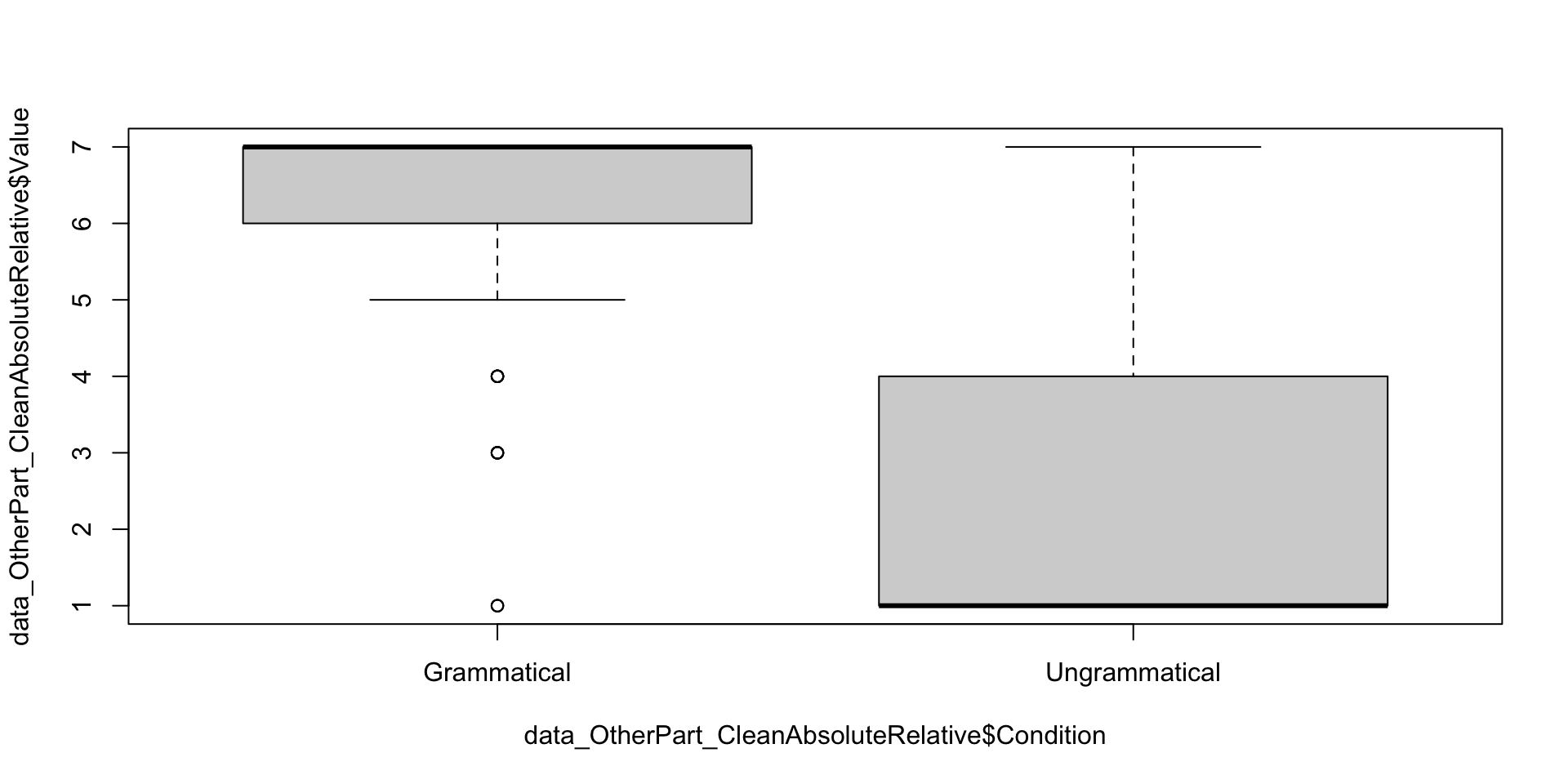
plot(data_OtherPart_CleanAbsoluteRelative$Value ~ data_OtherPart_CleanAbsoluteRelative$Condition)

summarySE(data_OtherPart_CleanAbsoluteRelative,
          measurevar = "Value",
          groupvars = "Condition")

      Condition   N    Value       sd        se        ci
1   Grammatical 144 6.361111 1.304168 0.1086807 0.2148283
2 Ungrammatical 142 2.485915 2.041193 0.1712931 0.3386347

3.1: Design-based analyses: Reaction time

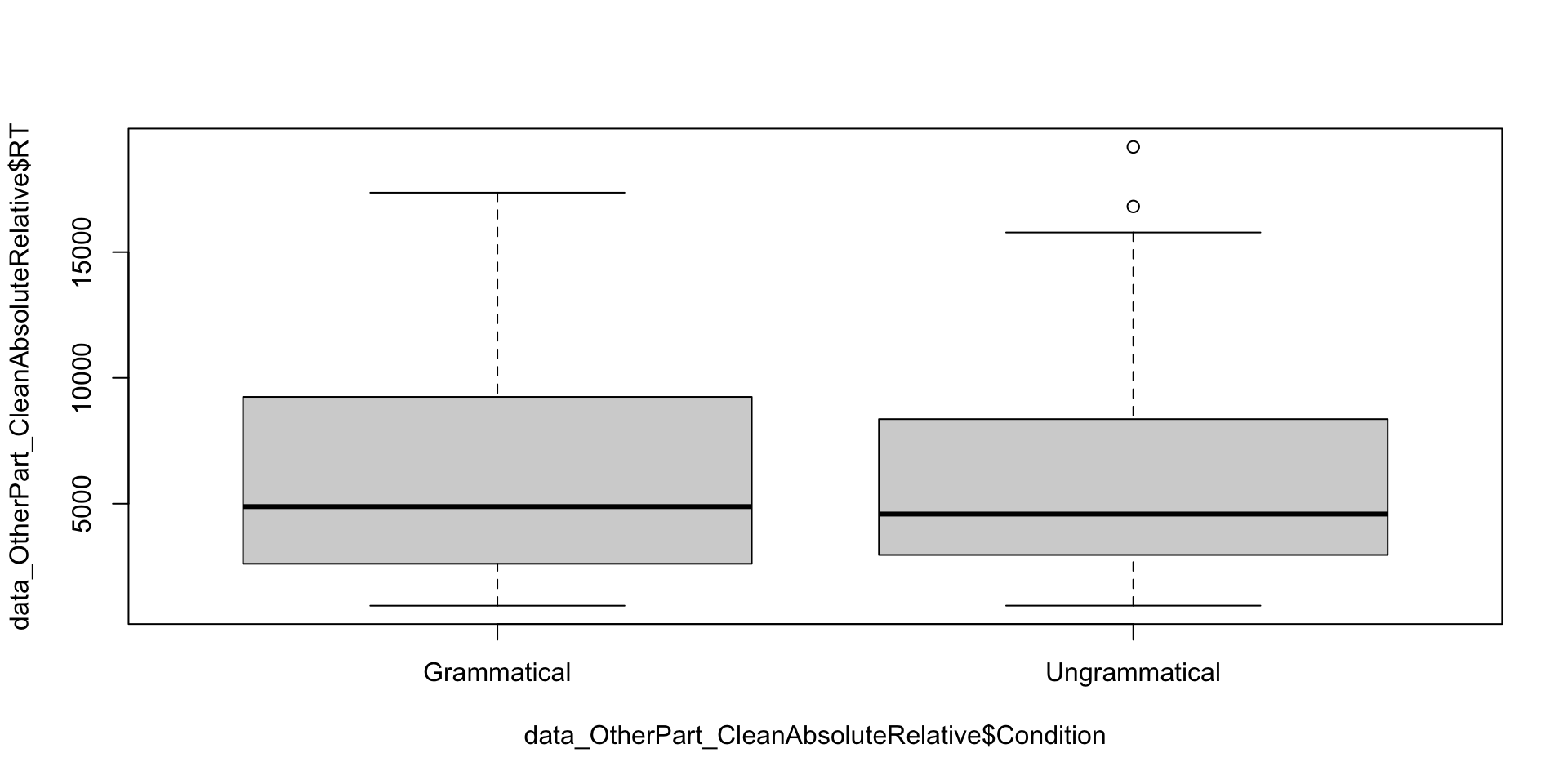
plot(data_OtherPart_CleanAbsoluteRelative$RT ~ data_OtherPart_CleanAbsoluteRelative$Condition)

summarySE(data_OtherPart_CleanAbsoluteRelative,
          measurevar = "RT",
          groupvars = "Condition")

      Condition   N       RT       sd       se       ci
1   Grammatical 144 6131.653 4240.087 353.3406 698.4457
2 Ungrammatical 142 6111.190 4277.881 358.9918 709.7022

3.2: Exploratory analyses

Why exloring the data?

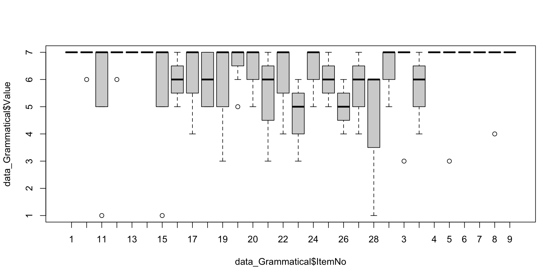
We observed more variation in the ungrammatical condition. The next step is to understand the source of such variation.

We already did our best with the participants, so it is likely to be related to the sentences.

3.2: Exploratory analyses, Grammatical condition

data_Grammatical <- droplevels(subset(data_OtherPart_CleanAbsoluteRelative,
                                        Condition == "Grammatical"))

plot(data_Grammatical$Value ~ data_Grammatical$ItemNo)

3.2: Exploratory analyses, Ungrammatical condition (1/3)

data_Ungrammatical <- droplevels(subset(data_OtherPart_CleanAbsoluteRelative,
                                        Condition == "Ungrammatical"))

plot(data_Ungrammatical$Value ~ data_Ungrammatical$ItemNo)

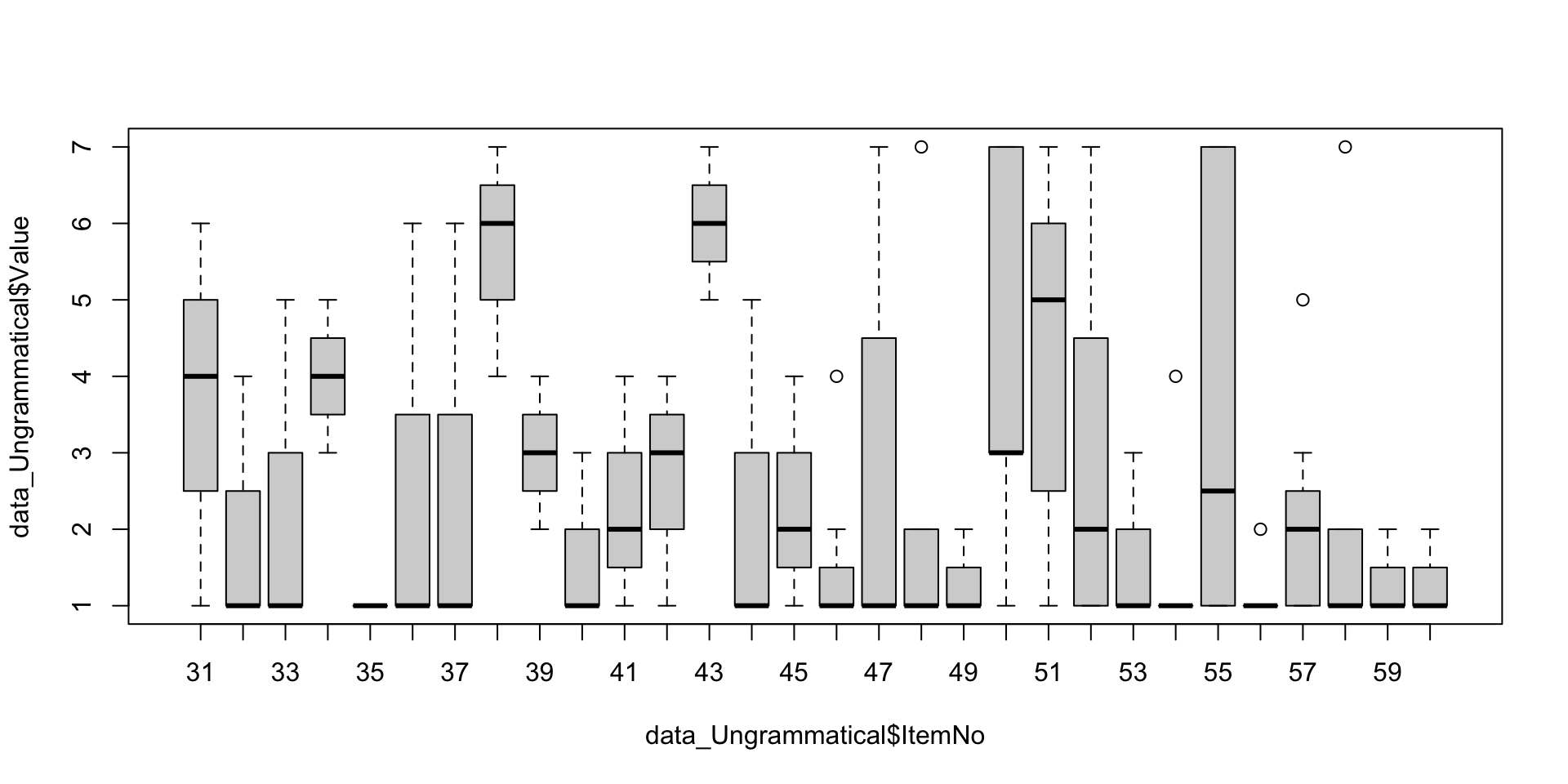
3.2: Exploratory analyses, Ungrammatical condition (2/3)

# Exploration of divergent ungrammatical sentences
data_Ungrammatical_OutlierValue <- subset(data_Ungrammatical, Value > 4)

data_Ungrammatical_OutlierValue_Summary <- droplevels(subset(data_Ungrammatical_OutlierValue,
                                                  select = c(ID_1_TimeReceived,
                                                             ItemNo,
                                                             Sentence)))
data_Ungrammatical_OutlierValue_Summary <- unique(data_Ungrammatical_OutlierValue_Summary)
data_Ungrammatical_OutlierValue_Overview <- table(data_Ungrammatical_OutlierValue_Summary$ItemNo)

data_Ungrammatical_OutlierValue_Overview


31 33 34 36 37 38 43 44 47 48 50 51 52 55 57 58 
 1  1  1  1  1  2  3  1  2  1  2  4  2  2  1  1

3.2: Exploratory analyses, Ungrammatical condition (3/3)

# Identify which ungrammatical sentences
data_Ungrammatical_OutlierValue_Overview <- as.data.frame(data_Ungrammatical_OutlierValue_Overview)
names(data_Ungrammatical_OutlierValue_Overview)[1] <- "ItemNo"

data_Ungrammatical_OutlierValue_Overview <- droplevels(subset(data_Ungrammatical_OutlierValue_Overview, Freq > 2))

data_Ungrammatical_OutlierValue_Overview <- left_join(data_Ungrammatical_OutlierValue_Overview, 
                                                      data_Ungrammatical, 
                                                      by = "ItemNo")
OutlierUngrammaticalSentences <- unique(data_Ungrammatical_OutlierValue_Overview$Sentence)
OutlierUngrammaticalSentences

[1] The bus stops not at this corner anymore
[2] It matters not what they think of us    
30 Levels: He needs not help with his homework today ...

📝 Assignment for next week

Important

Please annotate the Markdown file from this week, knit to a PDF file, and upload on Moodle!