Week 14 - Visualizing the data
CHC9012 | National Taiwan Normal University
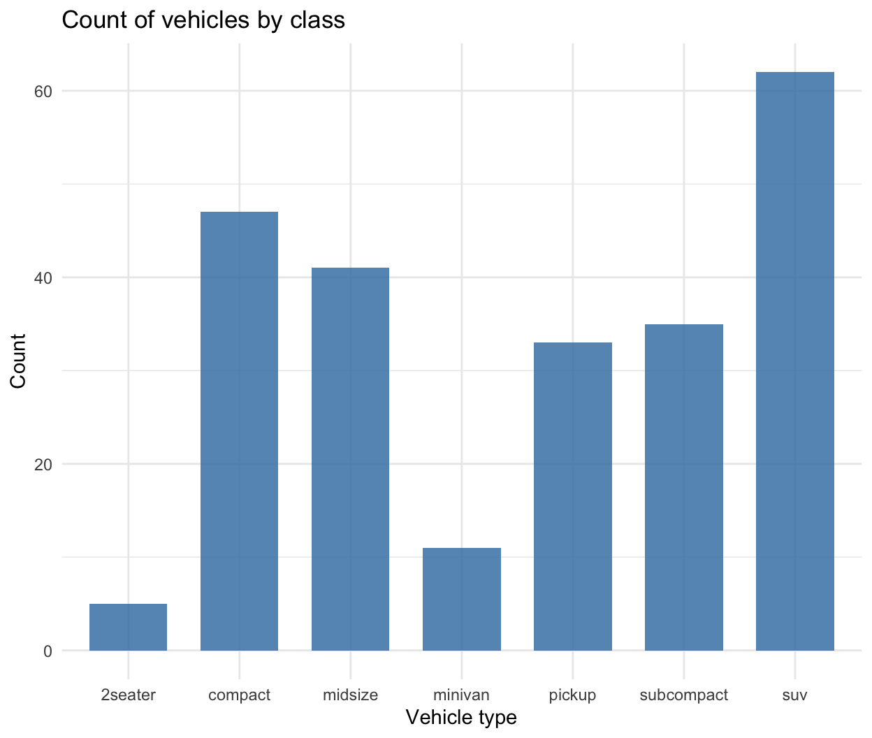
Bar plots for categorical counts
What it does:
Displays counts or frequencies of distinct categories.
Core question
Which categories are the most and least common in our dataset?
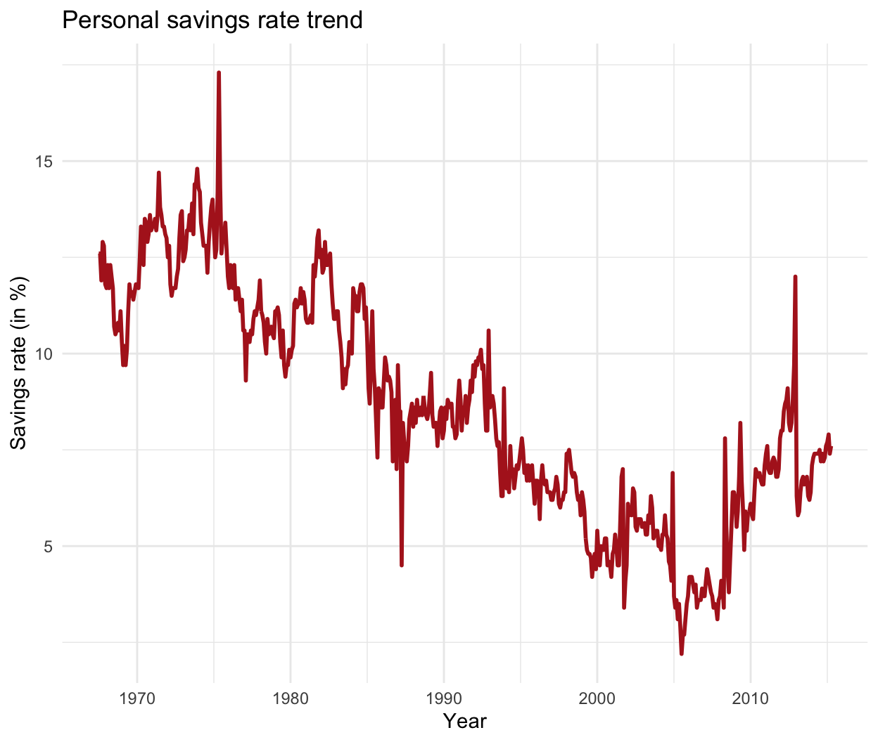
Line charts for continuous measurement, generally over time
What it does:
Connects individual data points chronologically or sequentially to reveal trajectories, spikes, or downward dips.
Core question
How is our metric moving over a continuous sequence?
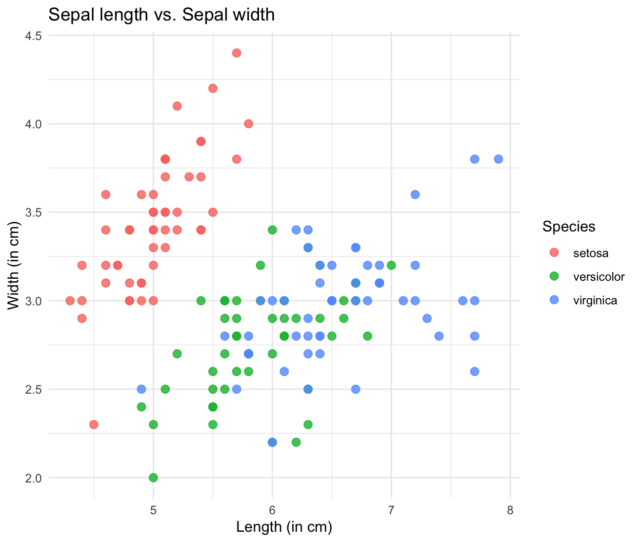
Scatter plots for relationships & correlations
What it does:
Plots individual data points at the intersection of two continuous numeric variables to display positive, negative, or non-linear correlations.
Core question
Does variable X increase, decrease, or remain unchanged as variable Y changes?
Combined plots for more complex data
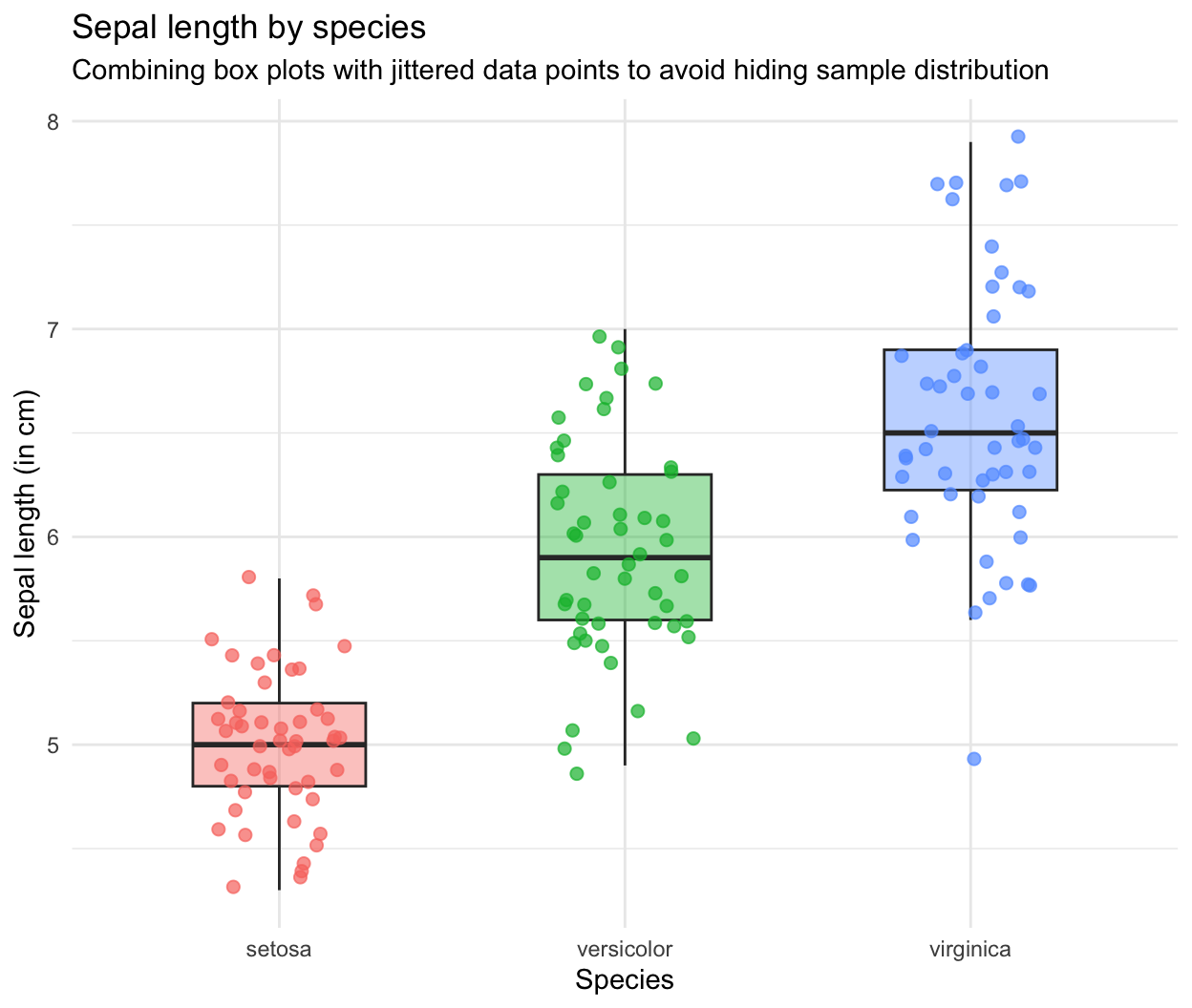
What it does:
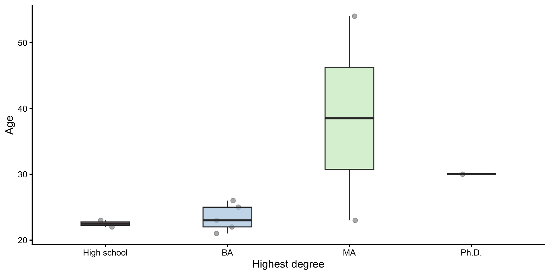
Plots two types of data at the same time.
Here, a boxplot with an additional scatter plot.
2.1 Introduction to ggplot2 and its spirit
Why using the ggplot2 package:
- Full control of what we want to plot
- Customization of the figure (legends, annotations, changing the theme and the colors, etc.)
The core spirit of ggplot2 is that any data visualization can be broken down into a series of independent layers stacked on top of one another.
Layer 1: Initialize
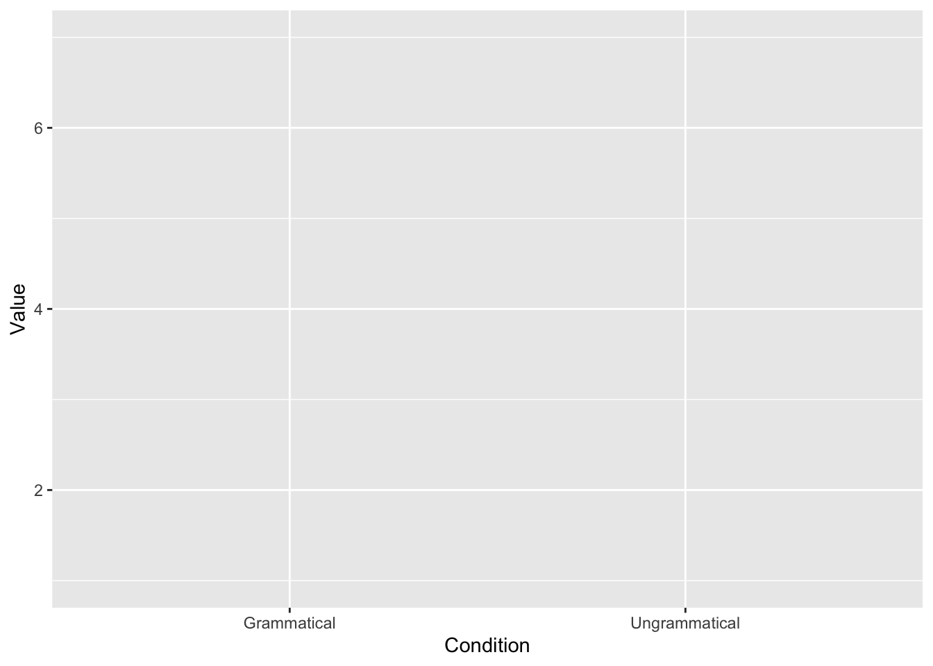
Step 1: Initialize
Create the empty canvas.

Layer 2: Aesthetics
Step 2: Indicate what to plot
In ggplot2 terms, this is called the ‘aesthetics’ (aes()).
Layer 3: Geometry
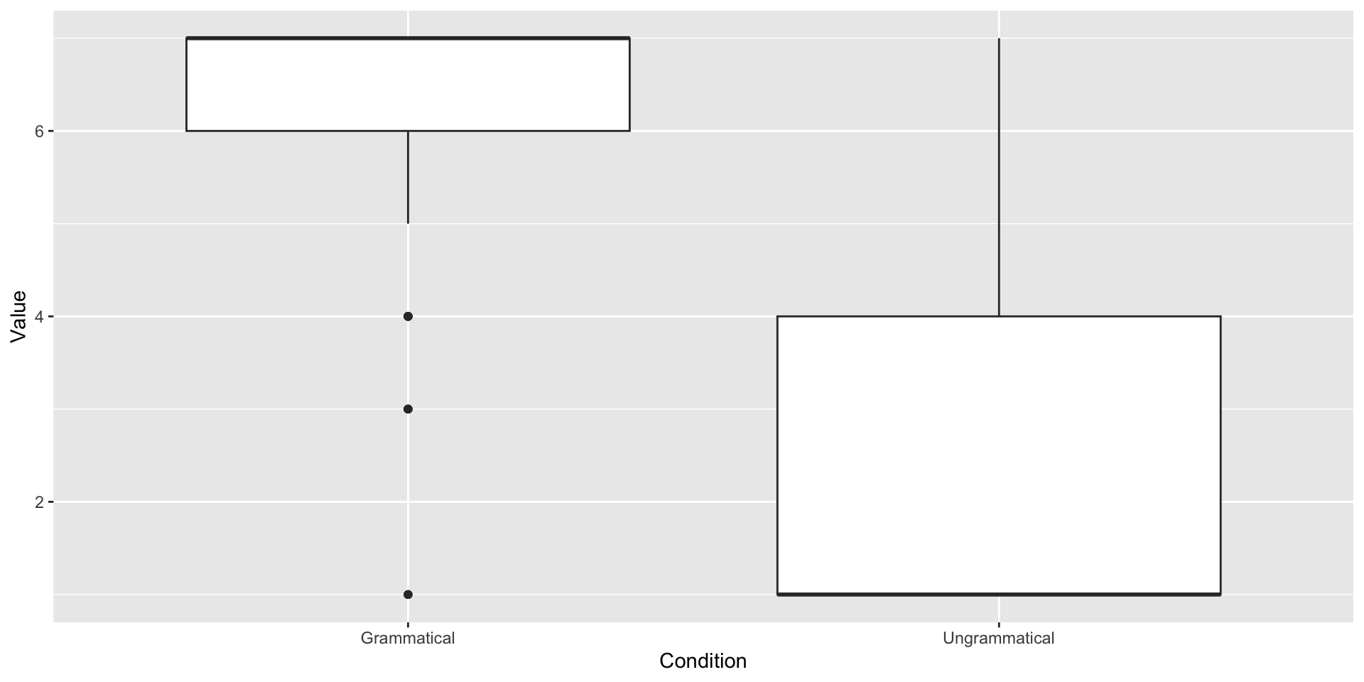
Step 3: Indicate how to plot
This is the step where you decide the kind of plot you want to use.
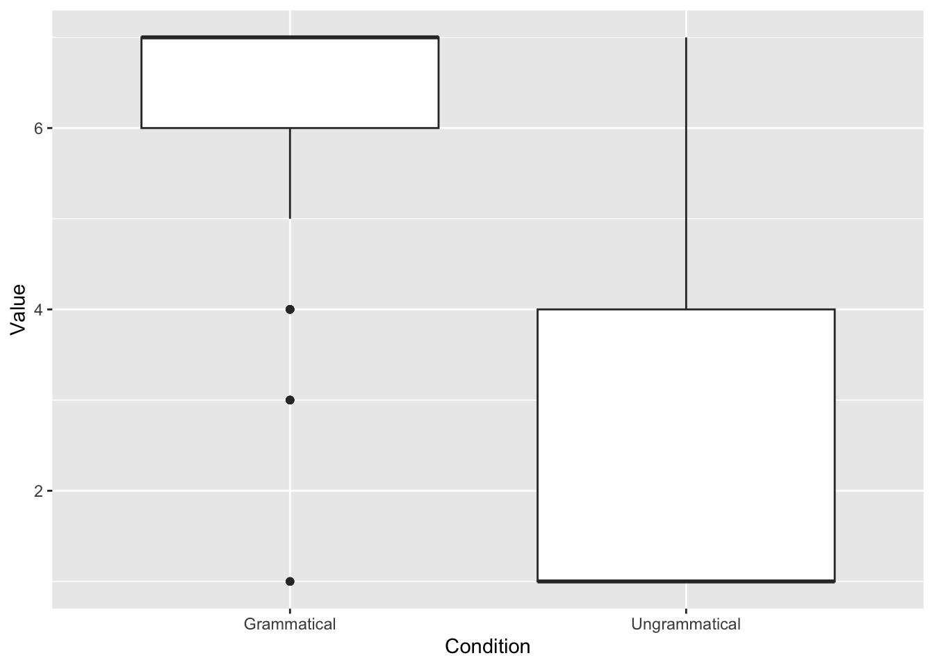
Layer 4: Polish
Step 4: Polish the details
Change the theme, the color, add a title (and subtitle), change the legend, the font style and size, etc.
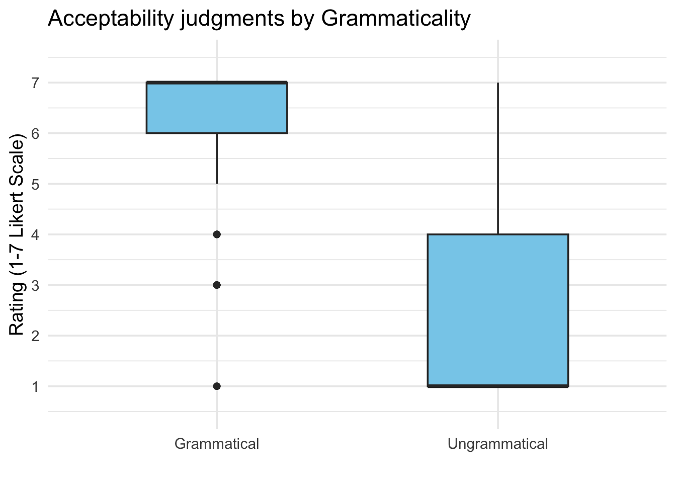
C. Create the canvas

D. Include what to plot (the “aesthetics”)
E. Include how to plot
F. Polish the details
ggplot(data_OtherPart_CleanAbsoluteRelative,
       aes(x = Condition,
           y = Value,
           fill = Condition)) +
  geom_boxplot(fill = "skyblue",
               width = 0.5) +
  labs(title = "Acceptability judgments by Grammaticality",
       x = "",
       y = "Rating (1-7 Likert Scale)") +
  theme_minimal(base_size = 14) +
  theme(legend.position = "none") +
scale_y_continuous(limits = c(0.5, 7.5),
    breaks = 1:7)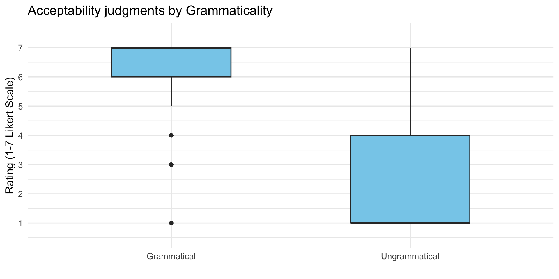
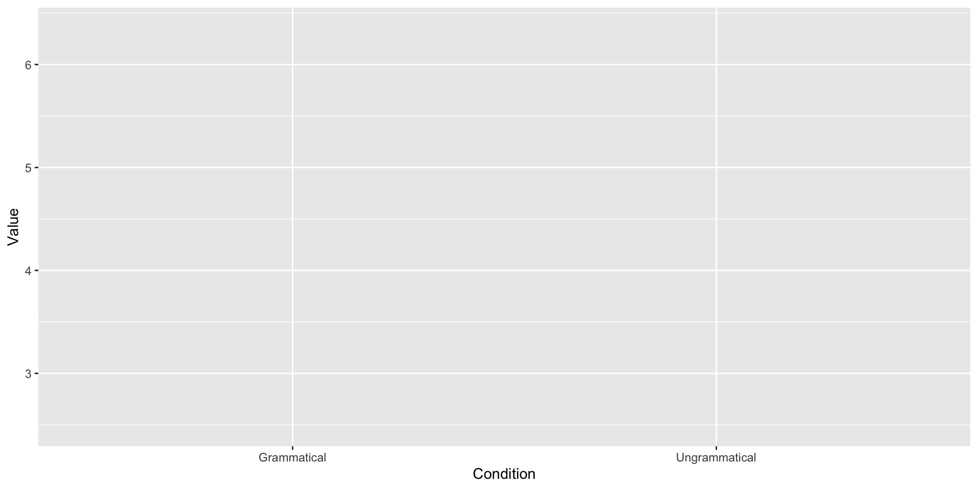
B. Create the canvas

C. Include what to plot (the “aesthetics”)
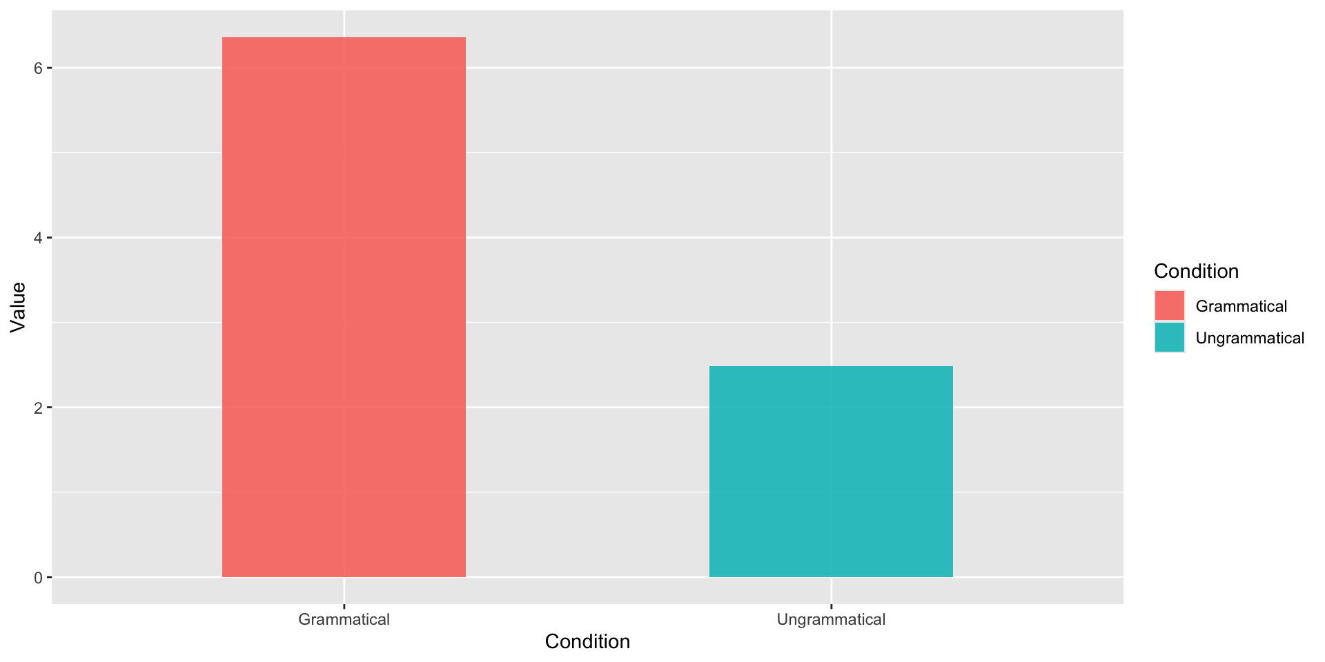
D. Include how to plot
E. Polish the details
ggplot(JudgSummary,
       aes(x = Condition,
           y = Value,
fill = Condition)) +
geom_col(width = 0.5, alpha = 0.9) +
geom_errorbar(aes(ymin = Value - ci,
ymax = Value + ci),
width = 0.15,
size = 0.7) +
geom_text(aes(label = round(Value, 2)),
vjust = 4,
color = "white",
size = 5,
fontface = "bold") +
scale_y_continuous(limits = c(1, 7),
breaks = 1:7,
oob = scales::rescale_none)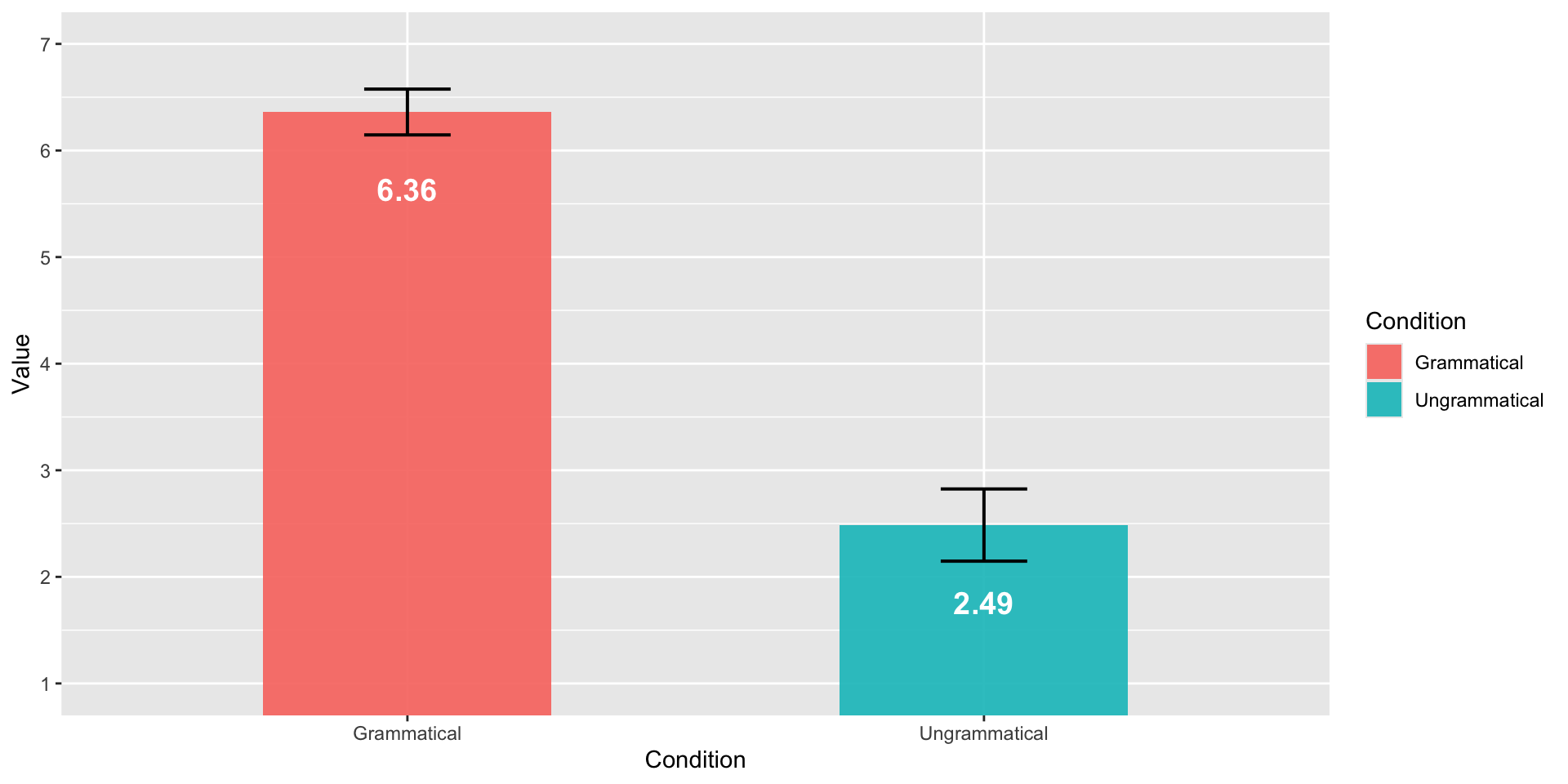
B. Create the figure
ggplot(JudgSummary,
       aes(x = Condition,
           y = Value,
           fill = Condition)) +
  geom_col(width = 0.5, alpha = 0.3) +
  geom_errorbar(aes(ymin = Value - ci,
                    ymax = Value + ci),
                width = 0.15,
                size = 0.7) +
  geom_text(aes(label = round(Value, 2)),
            vjust = 4,
            color = "black",
            size = 5,
            fontface = "bold") +
  scale_y_continuous(limits = c(1, 7),
                     breaks = 1:7,
                     oob = scales::rescale_none) +
  geom_jitter(data = JudgSummaryItem,
              aes(color = Condition),
              width = 0.2,
              height = 0.1,
              alpha = 0.5,
              size = 2.5) +
  theme_minimal(base_size = 14)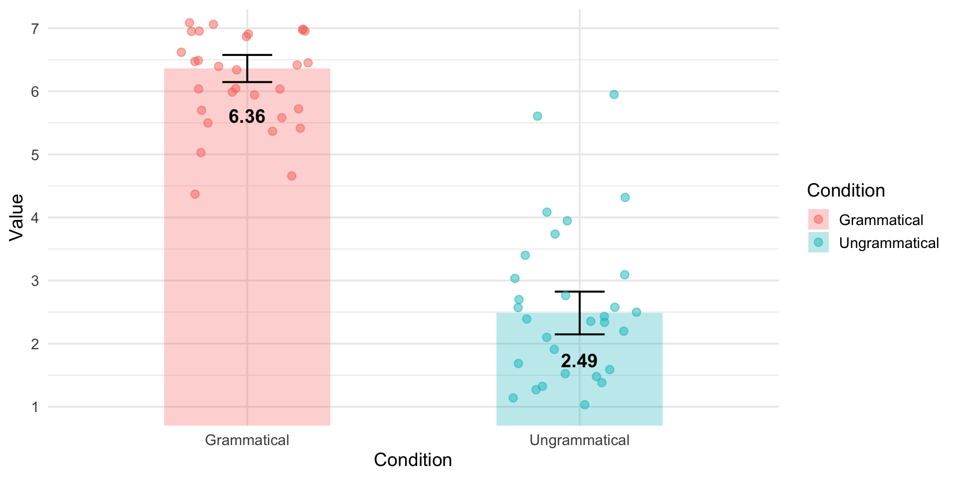
Reaction time: Box plots
No need to summarize the data with boxplots!
ggplot(data_OtherPart_CleanAbsoluteRelative,
       aes(x = Condition,
           y = RT,
           fill = Condition)) +
  geom_boxplot(fill = "skyblue",
               width = 0.5) +
  labs(title = "RT by Grammaticality",
       x = "",
       y = "Reaction time (in millisecond)") +
  theme_minimal(base_size = 14) +
  theme(legend.position = "none") +
scale_y_continuous(limits = c(0, 20000),
    breaks = seq(0, 20000, by = 4000))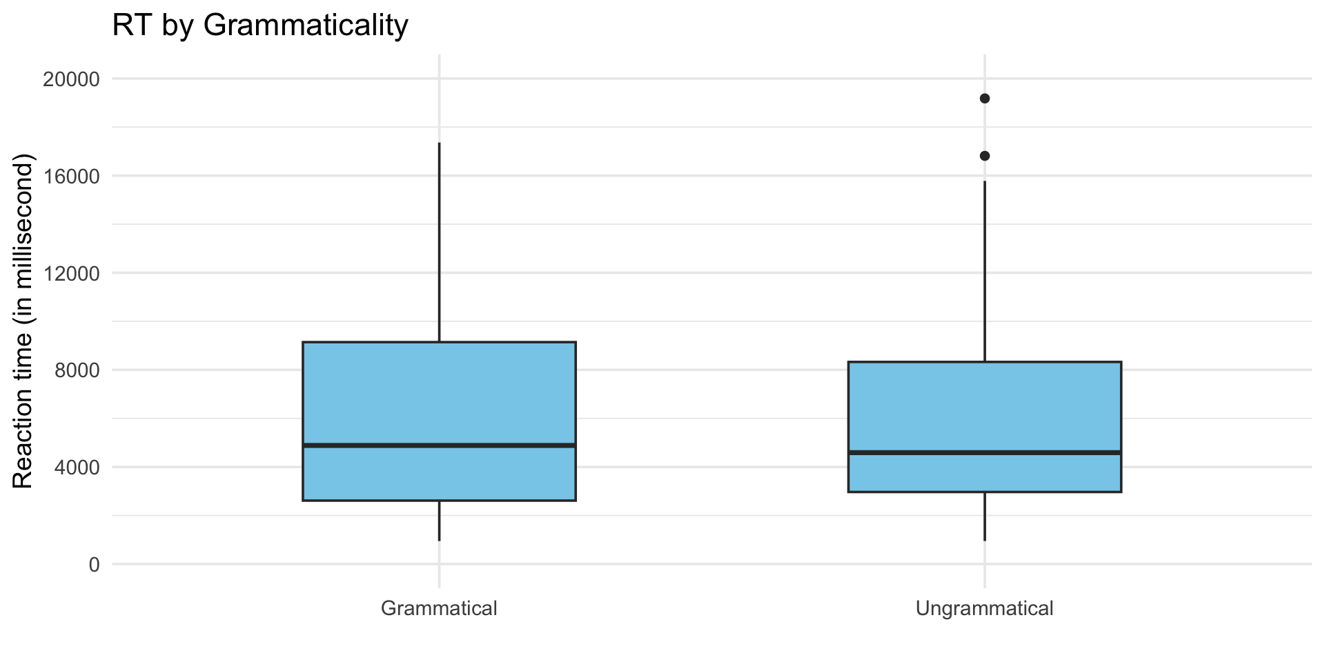
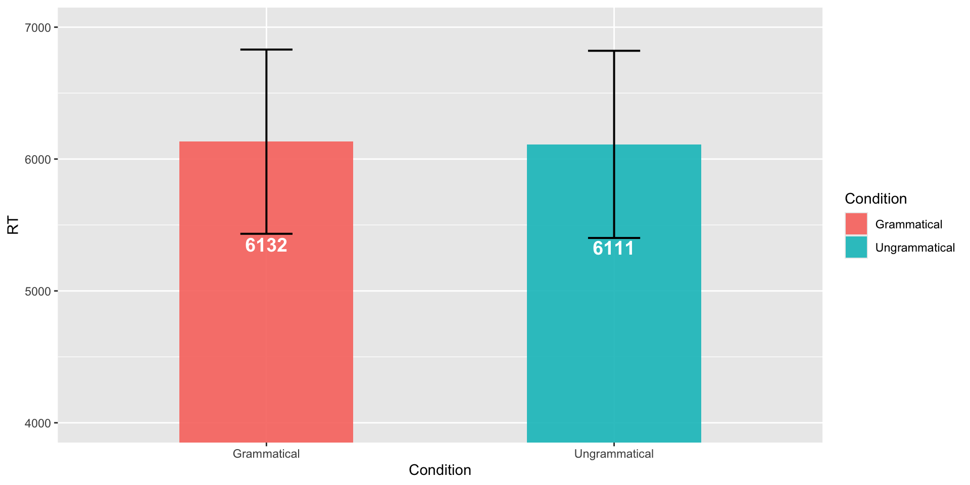
Reaction time: Bar plots
RTSummary <- summarySE(data_OtherPart_CleanAbsoluteRelative,
                       measurevar = "RT",
                       groupvars = "Condition")

ggplot(RTSummary,
       aes(x = Condition,
           y = RT,
           fill = Condition)) +
  geom_col(width = 0.5, alpha = 0.9) +
  geom_errorbar(aes(ymin = RT - ci,
                    ymax = RT + ci),
                width = 0.15,
                size = 0.7) +
  geom_text(aes(label = round(RT)),
            vjust = 8,
            color = "white",
            size = 5,
            fontface = "bold") +
  scale_y_continuous(limits = c(4000, 7000),
                     breaks = seq(4000, 7000, by = 1000),
oob = scales::rescale_none)| Condition | N | RT | sd | se | ci |
|---|---|---|---|---|---|
| Grammatical | 144 | 6131.653 | 4240.087 | 353.3406 | 698.4457 |
| Ungrammatical | 142 | 6111.190 | 4277.881 | 358.9918 | 709.7022 |
B. Create the figure
ggplot(RTSummary,
       aes(x = Condition,
           y = RT,
           fill = Condition)) +
  geom_col(width = 0.5, alpha = 0.3) +
  geom_errorbar(aes(ymin = RT - ci,
                    ymax = RT + ci),
                width = 0.15,
                size = 0.7) +
  geom_text(aes(label = round(RT)),
            vjust = 8,
            color = "black",
            size = 5,
            fontface = "bold") +
  scale_y_continuous(limits = c(3000, 9000),
                     breaks = seq(3000, 9000, by = 2000),
                     oob = scales::rescale_none) +
  geom_jitter(data = RTSummaryItem,
              aes(color = Condition),
              width = 0.2,
              height = 0.1,
              alpha = 0.5,
              size = 2.5) +
  theme_minimal(base_size = 14)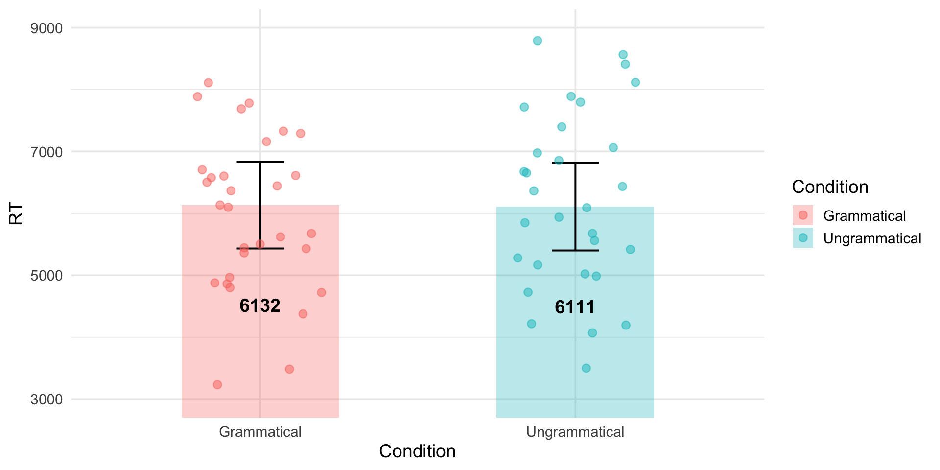
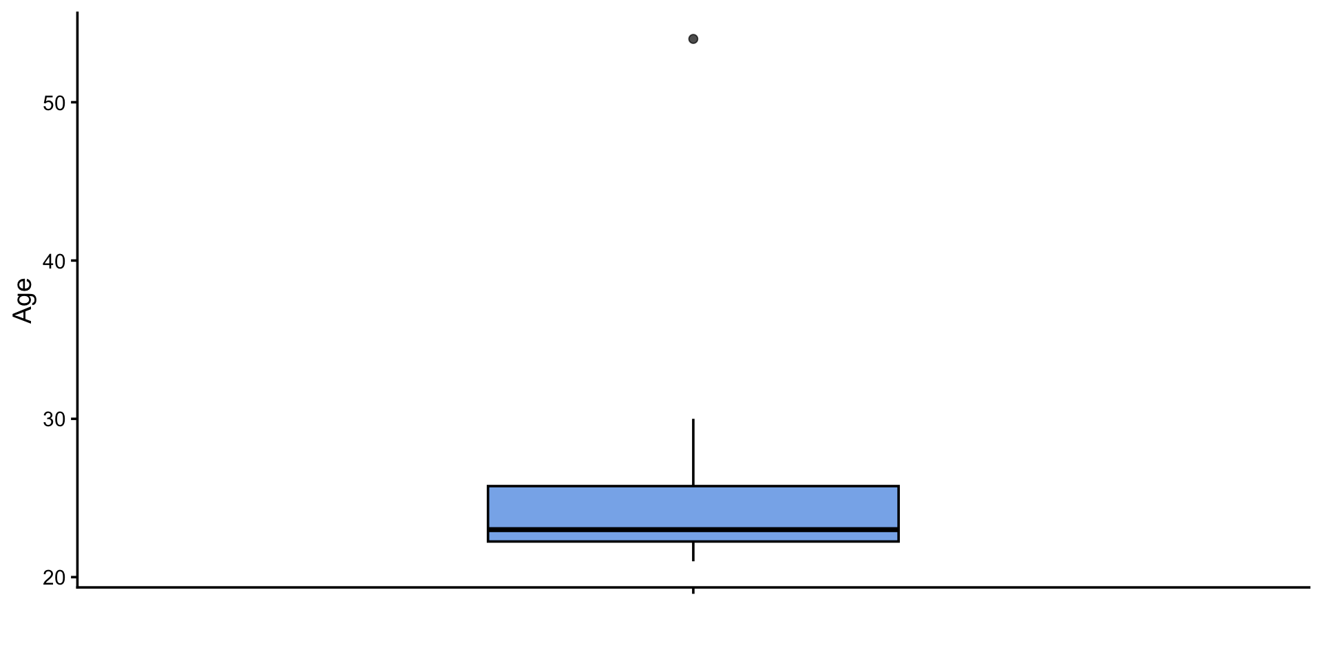
B. Plot the age of the participants
C. Plot the highest degree of the participants
ggplot(ParticipantBackground,
       aes(x = UserDegree,
           fill = UserDegree)) +
  geom_bar(width = 0.5,
           color = "black",
           alpha = 0.8,
           show.legend = FALSE) +
  geom_text(stat = "count",
            aes(label = after_stat(count)),
            vjust = -0.5,
            size = 5) +
  labs(x = "",
       y = "Number of participants") +
  scale_fill_brewer(palette = "Pastel1") +
  theme_classic(base_size = 14) +
  scale_y_continuous(expand = expansion(mult = c(0, 0.15)))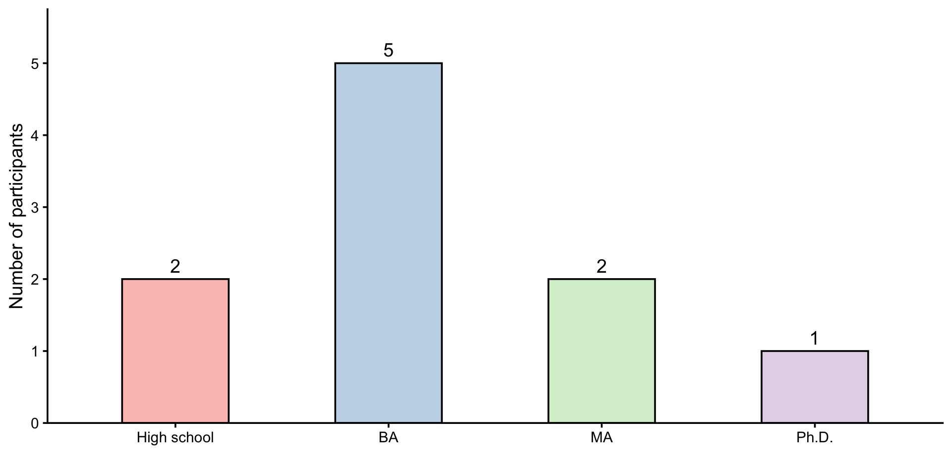
D. Plot the age and the highest degree of the participants at the same time
ggplot(ParticipantBackground,
       aes(x = UserDegree,
           y = UserAge,
           fill = UserDegree)) +
  geom_jitter(width = 0.1,
              height = 0,
              alpha = 0.5,
              size = 2.5,
              color = "dimgray") +
  geom_boxplot(width = 0.4,
               alpha = 0.7,
               outlier.shape = NA) +
  labs(x = "Highest degree",
       y = "Age") +
  scale_fill_brewer(palette = "Pastel1") +
  theme_classic(base_size = 14) +
  theme(legend.position = "none")